Equilibrium of the Firm and Industry under Perfect Competition

The article below offers an in-depth look at how firms and industries achieve equilibrium in a perfectly competitive market. By reading it, you will understand: 1. The definitions of firm and industry 2. The requirements for equilibrium in firms and industries 3. The short-run equilibrium for firms and industries 4. The long-run equilibrium for firms and industries.

Definitions of Firm and Industry:

Understanding the terms 'firm' and 'industry' is crucial before delving further into their analysis. A firm refers to an organization that creates and supplies goods demanded by consumers, aiming to maximize its profit.

According to R.L. Miller, "A firm is an entity that purchases and utilizes resources to sell goods and services." In Lipsey's view, "A firm is the entity that employs production factors to manufacture products for other firms, households, or the government."

An industry consists of a collection of firms that produce similar products within a market. Lipsey describes it as "a group of firms offering a specific product or closely related products." For instance, companies like Raymond, Maffatlal, and Arvind are textile manufacturers, and together they form the textile industry.

Equilibrium Conditions for Firms and Industries:

A firm reaches equilibrium when it has no inclination to modify its output level. It neither seeks to grow nor shrink, aiming instead to maximize profits by balancing marginal cost and marginal revenue, represented as MC = MR.

Visually, the equilibrium conditions for a firm can be outlined as follows:

(1) The marginal cost curve (MC) must intersect with the marginal revenue curve (MR). While this is a necessary condition, it does not guarantee that the firm is at equilibrium.

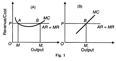
(2) The MC curve should intersect the MR curve from below, and above the equilibrium point, the MC curve must remain above the MR curve. In perfect competition, a firm’s MR curve aligns with its average revenue (AR) curve, appearing horizontal along the X-axis. This means a firm achieves equilibrium when MC = MR = AR (Price).

In Figure 1(A), the MC curve first meets the MR curve at point A. This fulfills the MC = MR condition, but it does not indicate maximum profit since beyond point A, the MC falls below the MR. Thus, producing less than output OM isn’t wise when the firm can earn higher profits by exceeding this output level

Point B represents the maximum profit point where both conditions hold. Between points A and B, increasing output is beneficial as MR exceeds MC. Production will cease when the firm reaches the OM1 output level where it meets both equilibrium conditions.

If an organization intends to create output exceeding OM1, it will face losses, as the marginal cost surpasses the marginal revenue after the equilibrium point B. This conclusion also applies when observing a straight-line marginal cost (MC) curve, as illustrated in Figure 1.

An industry reaches equilibrium when there is no motivation for companies to enter or exit the market, and each individual company is in a state of balance. The first condition means that the average cost (AC) curves align with the average revenue (AR) curves of all firms within that industry. At this point, firms only earn normal profits, which are factored into their average cost curves.

The second condition indicates that the marginal cost (MC) equals marginal revenue (MR). In a perfectly competitive market, both of these conditions must be met at the equilibrium point, which can be expressed as follows:

MC = MR … (1)

AC = AR … (2)

AR = MR

MC = AC = AR

This scenario depicts a complete equilibrium for the industry.

Short-Run Equilibrium of the Firm and Industry:

In the short run, a firm is in a state of equilibrium when it neither wants to increase nor decrease its production, aiming instead for maximum profit or minimal losses. The short run refers to a timeframe where the company can adjust its output by altering its variable production factors. During this period, the total number of firms in the market remains constant since existing firms cannot exit, nor can new firms enter.

Assumptions:

The following points form the basis of this analysis:

1. All companies utilize the same production factors.
2. Companies exhibit varying levels of efficiency.
3. Cost curves differ across firms.
4. Each company sells its products at a uniform price set by industry supply and demand, indicating that each firm's price (P) is equal to average revenue (AR) and marginal revenue (MR).
5. Firms produce and sell different amounts.

The concept of short-run equilibrium for a firm can be understood through marginal analysis and total cost-total revenue analysis.

(1) Marginal Cost-Marginal Revenue Analysis:

In the short run, a firm will continue production only if its price meets or exceeds the average variable cost (AVC). Additionally, when the price surpasses the short-run average costs (SAC or ATC), represented as P - AR > SAC, the firm achieves supernormal (or abnormal) profits.

If the price matches the average total costs, specifically P = AR = SAC, the firm earns normal (or zero) profits, effectively breaking even. Conversely, if the price aligns with AVC, the firm experiences a loss. Should the price dip below AVC, the firm will cease operations because it must at least cover its AVC to produce in the short run.

Therefore, under perfect competition, a firm reaches equilibrium in all aforementioned scenarios. These are illustrated below in graphical form.

Supernormal Profits:

Supernormal profits arise in the short run when the price exceeds the short-run average cost, as depicted in Figure 2 (A). The firm is at equilibrium at point E1, where SMC equals MR and the SMC curve intersects the MR curve from below. OQ represents the output at equilibrium, while OP (= Q1E1) indicates the equilibrium price. The average costs for the short run are represented by Q1S.

The profit per unit, illustrated as SE1 (= Q1E1 - Q1S), contributes to total supernormal profits, calculated as TS (equilibrium output) multiplied by the per-unit profit, which corresponds to the area TSE1P.

Normal Profits:

When the price equals the short-run average costs, as shown in Figure 2 (B), the firm can earn normal profits. The equilibrium is reached at point E2, where SMC equals MR, with the SMC curve intersecting MR from below. OQ2 indicates equilibrium output, while OP (= Q2E) denotes the equilibrium price. Normal profits occur since Price equals AR, MR, SMC, and SAC at the minimal point E2.

Minimum Loss:

The firm can be at equilibrium and still face losses if the price falls below short-run average costs, as depicted in Figure 2 (C). Equilibrium is at point E3, where SMC equals MR, and the SMC curve intersects the MR from below. The equilibrium output is OQ3, while OP (= Q3E3) is the equilibrium price.

Given that the average costs marked as Q3B exceed the price at Q3E3, the loss per unit is represented as E3B (Q3B - Q3E3). Total losses are calculated as the area PE3 x E3B = PE3BA. The firm will sustain production at output OQ3 as long as it covers its average variable costs along with a portion of its fixed costs.

Maximum Loss:

When the price, as illustrated in figure 2, drops to the average variable cost (AVC), the company manages to cover its AVC, reflected at point D in figure 2. At this stage, the firm is indifferent between continuing operations or shutting down, as its losses are at their peak.

In the short term, it is advantageous for the firm to keep producing at output level OQ4, even if it faces losses represented by PE4GF, instead of ceasing production. OQ4 represents the output level where the firm would consider shutting down; below price OP, production will halt. Thus, E4 serves as the shutdown point.

Shut Down Stage:

In Figure 2 (E), a firm finds itself unable to even cover its AVC at the output level of OQ0, since the price OP lies below the AVC curve, necessitating a shutdown.

In the short run, firms may experience normal profits, supernormal profits, or sustain losses.

Total Cost-Total Revenue Analysis:

The firm’s short-run equilibrium can also be analyzed using total cost (TC) and total revenue (TR) curves. Profit maximization occurs when the difference between TR and TC is at its highest, as depicted in Figure 3, where TR is the total revenue line and TC denotes total costs.

The TR curve rises as a straight line starting from the origin. This trend occurs because, in perfect competition, the firm can sell varying quantities of its product at a stable price. If no product is produced, the total revenue remains zero. An increase in production leads to an increase in total revenue, establishing a linear and upward-sloping TR curve.

Profit maximization for the firm happens at the output level where the gap between TR and TC is largest. Geometrically, this occurs where the slope of a tangent to the total cost curve matches the slope of the total revenue curve. In Figure 3, the maximum profit is noted at point TP for output OQ.

If the output deviates from OQ, either lower or higher, between points A and B, profits diminish. At output level OQ1, the firm experiences maximum losses, as the TC curve exceeds the TR curve, resulting in zero profit at Q1.

This point marks the firm’s break-even threshold. Once it surpasses output level OQ1, it begins to earn profits, although at output level OQ2, profits again drop to zero. Beyond this point, losses will occur since TC will once again exceed TR.

Short-Run Equilibrium of the Industry:

An industry reaches short-run equilibrium when its total production remains constant, without tendencies to increase or decrease output. When all firms are in equilibrium, the entire industry achieves equilibrium. For the industry to exhibit full equilibrium in the short run, every firm must only generate normal profits.

The requirement for this situation is that SMC should be equal to MR, AR, and SAC. However, the complete equilibrium of the industry often occurs by coincidence because, in the short run, some businesses may be making excess profits while others may be facing losses. Nonetheless, short-run equilibrium exists in the industry when the quantity demanded matches the quantity supplied at the price that balances the market.

This is demonstrated in Figure 4, where Panel (A) shows industry equilibrium at point E, where the demand curve D and the supply curve S meet, setting the price OP, which allows for the total output OQ to be sold. Meanwhile, at this OP price, certain firms enjoy excess profits PE1ST, as seen in Panel (B), while other firms experience losses represented by FGE2P in Panel (C) of the figure.

Long-Run Equilibrium for Firms and Industry:

In the long run, firms have the flexibility to alter their operational scale and facilities. During this period, all costs are variable, eliminating fixed costs. A firm achieves long-run equilibrium in a perfectly competitive environment when it has no desire to alter its output level.

At this stage, firms earn normal profits. If some firms profit excessively, it triggers the entry of new firms into the market, pushing down those supernormal profits. Conversely, if any firms incur losses, some will exit the industry until only normal profits remain.

Consequently, there is no pressure for firms to enter or exit the industry, as every firm is set to earn normal profits. "In the long run, firms reach equilibrium when they adjust their operations to produce at the lowest point of their long-run AC curve, which touches the demand (AR) curve determined by market pricing,” allowing them to secure normal profits.

Assumptions:

This examination is founded on several assumptions:

1. Firms can freely enter and exit the industry.

2. All firms possess equal levels of efficiency.

3. All factors of production are identical and can be acquired at stable and uniform prices. SMC

4. The cost curves of firms are consistent.

5. Firms have equivalent plants, sharing the same technology.

6. All firms possess complete knowledge of pricing and output conditions.

Under these assumptions, each firm in the industry achieves long-run equilibrium when it meets two key criteria.

(1) In equilibrium, its short-run marginal cost (SMC) must align with its long-run marginal cost (LMC), as well as its short-run average cost (SAC) and long-run average cost (LAC), with all equating to MR = AR = P.

The first condition for equilibrium can be stated as:

At its lowest point, SMC equals LMC, MR, AR, P, SAC, and LAC.

Additionally, the LMC curve must intersect the MR curve from underneath. These equilibrium conditions are fulfilled at point E, as shown in Figure 5. Here, both SMC and LMC curves approach the SAC and LAC curves from below at their minimum point E. Moreover, they intersect the AR = MR curve from below. At this point E, all curves converge, enabling the firm to produce the optimal output OQ and sell it at the price OP.

Assuming that all firms within the industry have equal costs, long-term equilibrium is achieved. At the price OP, no firm has the motivation to exit or enter the industry, allowing all firms to earn normal profits.

Long-Run Equilibrium of the Industry:

In the long run, an industry's equilibrium occurs when all firms are making normal profits. This situation creates no reasons for firms to leave or for new firms to join. With homogenous factors, consistent prices, and the same technology, each individual firm and the industry as a whole reach a state of equilibrium characterized by LMC equaling MR and AR (minus P) equaling LAC, all at their minimum levels.

This equilibrium is reached when the long-term price for the industry is established through the balance of total industry demand and supply.

Figure 6 (A) illustrates the long-run equilibrium of the industry, with the long-run price OP determined where the demand curve D intersects the supply curve S at point E. At this intersection, the industry produces output OM. At the price OP, the firms are stable at point A in Panel (B) with an output level of OQ, where LMC, SMC, MR, and P (or AR) equal SAC and LAC at their lowest point.

At this level, firms achieve normal profits and feel no urge to either enter or exit the industry. Consequently, when the industry reaches long-run equilibrium, each firm within it also achieves the same state. If both the industry and firms are in long-run equilibrium, it naturally follows that they are also in short-run equilibrium.

---------------------------------------------------------------------------------------------------------